home & schedule | syllabus | contact | grades

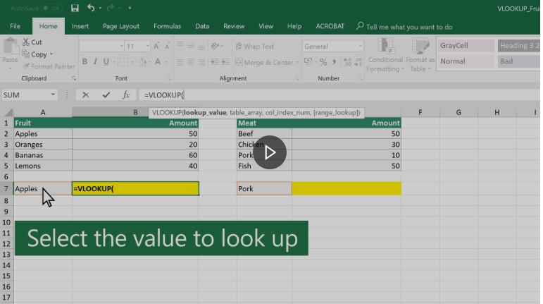
VLOOKUP is an Excel function to lookup and retrieve data from a specific column in table. It is an Excel way to do what SQL can do with a relational database.

What is VLOOKUP?

It's an Excel function that one may use when one needs to find things in a table or a range by row. For example, look up a price of an automotive part by the part number, or find an employee name based on their employee ID.

In its simplest form, the VLOOKUP function says:

=VLOOKUP(What you want to look up, where you want to look for it, the column number in the range containing the value to return, return an Approximate or Exact match – indicated as 1/TRUE, or 0/FALSE).

Still using your downloaded workbook ...

We will demonstrate practice with the VLOOKUP function

You won't have to do VLOOKUP for the task, but it might be useful to see it work for you.

In this workbook, composed of two worksheets, we want to use a lookup table on the 11-Calendars worksheet to populate data in column D on 12-Fall 2020 Class Schedule worksheet

1. select cell D2 on the 12-Fall 2020 Class Schedule
2. in the  formula bar , insert this formula
   (use your CNTL+C or CMD+C to copy it from this web page, and your CNTL+V or CMD+V to paste it in the cell)

=VLOOKUP(E2,11-Calendars!$F$4:$G$11,2,FALSE)

This means

• the value in this cell equals
• the value you will find when you use this function to
• compare the value in the same line and one cell to the right on this worksheet,
• to the values in the array of cells on the 11-Calendars worksheet in the absolute range of cells from cell F4 through G11,
• where it will look for a value that matches the value in cell E2 in this worksheet in column cells F4 through F11 on the Calendars worksheet,
• and find the value that resides in the related cell G4 through F11 on the 11-Calendars worksheet,
• and insert that value back into this cell

Once you have the value in cell D2, you can use the  fill handle  and drag down the function from D2 to D84. The function will continue to match the value in the relative column E cell to the absolute values in cells F4 through F11 on the 11-Calendars worksheet and return the related value from cells G4 through G11 and place them in cells D2 through as far as you drag down the function.

Note, when using the  fill handle , you drag down all the cell, to include the color formatting of the cell as well as the function within the cell.

week of 05 November labs | VLOOKUP | SQL creation