Using spreadsheets as databases

[top]
Sorting
Your data is entered into your database, row by row, in any order. Should you wish to re-order the rows to better portray some aspect of the database, you may wish to sort the data. There are multiple ways to do it (use this example).
- Sort list in alphabetical, numerical, or chronological order
- Order can be ascending or descending
How to sort
Select the column or array you wish to sort, then choose Data > Sort & Filter > Sort from the ribbon
![[select the array to be sorted, then select the sort tool from the ribbon]](images/spreadsheets.sort.ribbon.png)
Or use the sort tools from the right click option.

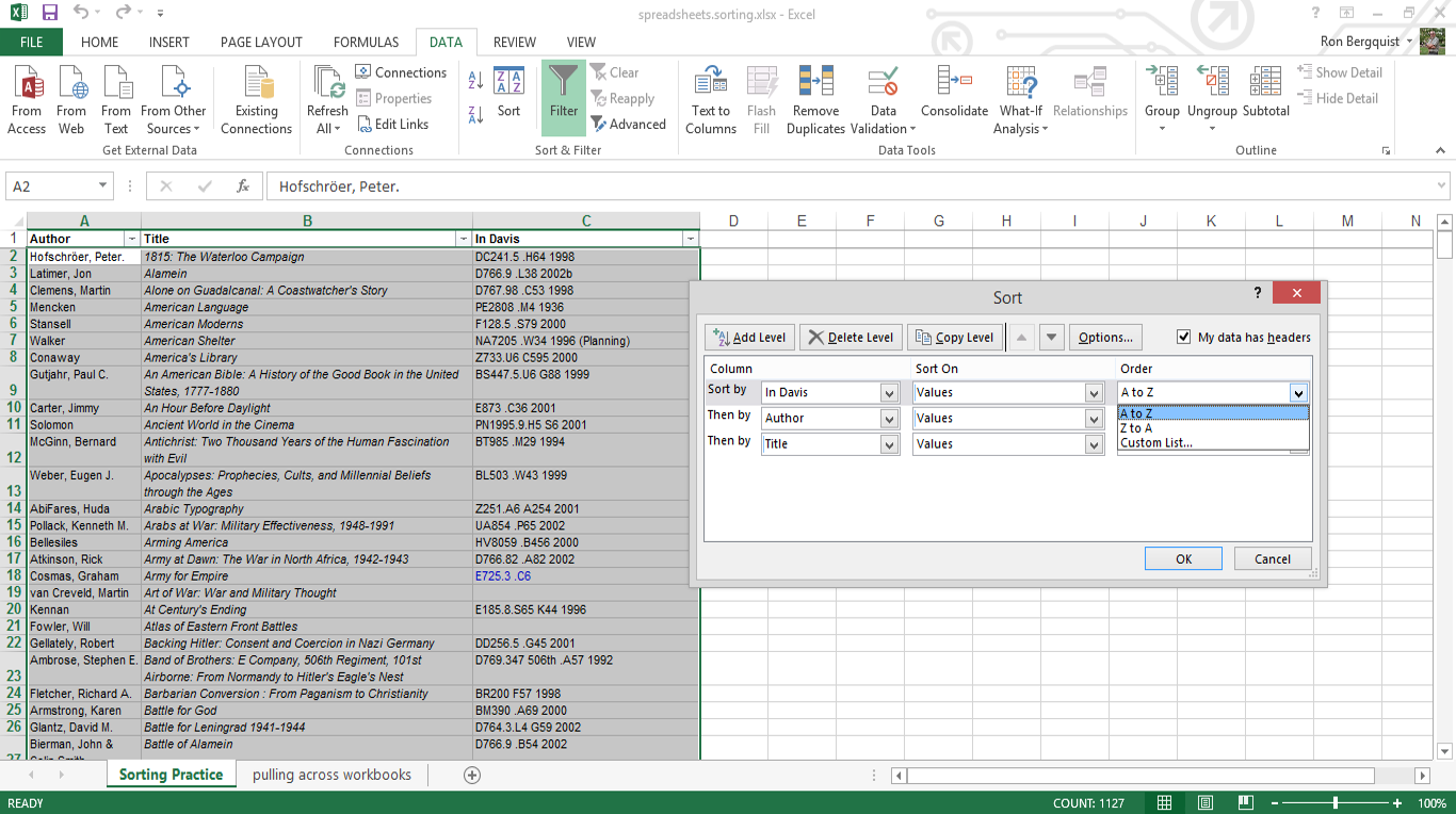
The ribbon option and the Custom Sort option both will reveal the dialog box.
![[MSExcel 2007 sort dialog box]](images/spreadsheets.sort.dialog_box.png)
Check that the data sorted correctly. To undo, use the undo icon or CTRL-Z or "Edit, Undo" or just redo the sort.
[top]
Filtering
Filtered data displays only the rows that meet criteria (or "Conditions you specify to limit which records are included in the result set of a query or filter") that you specify and hides rows that you do not want displayed. After you filter data, you can copy, find, edit, format, chart, and print the subset of filtered data without rearranging or moving it.
You can also filter by more than one column.
Filters are additive, which means that each additional filter is based on the current filter and further reduces the subset of data.
Use to filter through only those records of a database that meet specific criteria, such as asking the tool to retrieve only those records that begin with the letter "S". (use this example).
How to filter
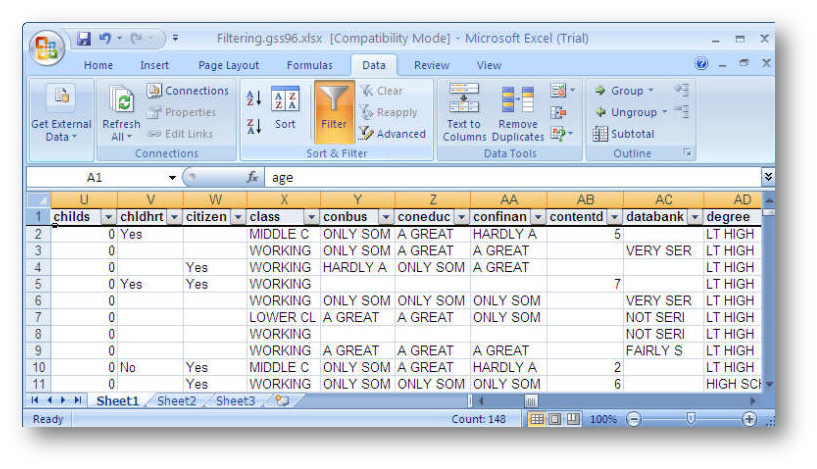
Select Data > Sort & Filter > Filter from the ribbon. The filter will be applied to the column headings (which define the data in the rows below the heading row.

Using the Drop Down filter menu, select the entry that you wish to filter for (the result will hide all by the rows that include the filter term). It will either look down the column and filter for the value it finds, or will allow you to create a custom filter for values you define.
![[filter options from the drop down button on the header row]](images/spreadsheets.filter.options.png)
You can also create Custom filters (to do Boolean searches, for example). A dialog box will appear. If the values in the column are text, the filter will be a text filter. If they are numerical, the filter will be a number filter.
![[custom filter dialog box]](images/spreadsheets.filter.custom.dialog_box.png)
Use the drop down menus (or type in) the filter you want.
Use filters to arrange data for charting or printing
Once you have filtered, you can create a chart based only on the displayed data. When you print, only the displayed rows will appear in the printed version (because the other rows are hidden). Should you choose to do additional formatting after having filtered, formatting commands will only affect the visible cells.
[top]
Subtotals
You can have Excel calculate subtotals or totals for portions of your worksheet data. For example, in a worksheet with data for three different categories, you can first sort the products by category, and then select all the cells that contain data and have Excel place subtotals beneath each category range and a grand total beneath the entire range of selected categories.
Entering a subtotal (use this example).
Sort the data according to the order in which you want to create subtotals. To generate subtotals based on category, for example, first sort the list by the desired category.
Select the array you want to summarize, choose Data > Outline > Subtotal to get the Dialog Box. You will have to have a repeating value in some column so that the Subtotal tool can subtotal each time that repeating value changes.
In the Dialog box, select the group to define the subtotals
![[subtotal data array in Excel 2007]](images/spreadsheets.subtotal.tool.png)
to generate automatic subtotals by date, for example, select the Date field from the At Each Change in drop-down list
![[subtotal function option in dialog box]](images/spreadsheets.subtotal.dialog_box.02.png)
if you want to Sum, select the Sum function from the Use Function drop-down list (there are other functions you may wish to use in this drop-down box)
![[add subtotal to option in dialog box]](images/spreadsheets.subtotal.dialog_box.03.png)
Choose the data you want to subtotal in the Add Subtotal To box. To subtotal the data found in a certain field, for example, select that field.
Press Enter or choose OK to add the subtotals to your list.
Removing subtotal data from a list
Select a cell in the subtotaled list and choose the Data > Subtotals command. Choose the Remove All button from the Subtotals dialog box.
[top]
Linking within worksheets or between workbooks
Among Worksheets within a Workbook
One can pull data from cells that occur on different worksheets (in this case looking at gas and water simultaneously).
![[create a new window in a workbook and arrange to view both at once]](images/spreadsheets.view-multiple-worksheets.png)
Start with
=,
then select either a
location
or select a
function.
Click the first sheet and then select appropriate cell(s)
Holding the shift key, click the second (or third, fourth) sheet(s)
Press Enter (can be done manually)
- results in ='Auto Mileage'!A91-'Auto Mileage'!A3
- or with functions =('Auto Mileage'!C91)/SUM('Auto Mileage'!E3:E91)
Notice the range in the formula "sum of gallons used" =SUM('Auto Mileage'!E63:E91)
Among Workbooks
Use View > Window > Arrange All to view multiple Workbooks (in this case, look at Sorting, charting, and formulas).
![[view multiple workbooks simultaneously to work with them]](images/spreadsheets.view-multiple-workbooks.png)
Enter formula (or function) using formula bar = sign, then select the function type (e.g., SUM) to open dialog box. Move dialog box if necessary. Place cursor in dialog box next to "Number one", then select appropriate cell(s) on linking sheet in linking workbook. Repeat for "Number two" and so forth, until you have selected all the cells you wish to link. When finished, press OK.
Example of formula:
=MAX('[Formulas_practice.xlsx]Adding_formulas'!$I$10:$I$13)/AVERAGE([charting_practice.xlsx]dat00_eu!$B$1550:$B$1572)
[top]

