Tools for Information Literacy | Week ⑪ 
Facility with functions

Use functions to pull data from a second worksheet to create new data

Why we do this	What we are to do
to demonstrate facility with functions and formatting of the resultant data	On the 05-Summary worksheet, in cell B4 enter the words "Earliest Foundation Date." In cell K4 insert a function that will return the earliest foundation date from the data in the FC = Foundation century column (that would be column G) on the 02-CONDITIONAL FORMATTING worksheet. Remember, these numbers represent years and so should not be displayed with any decimal places.
to demonstrate facility with functions and formatting of the resultant data	On the 05-Summary worksheet, in cell B6 enter the words "Total number of counties in the US." In cell K6 insert a function that will return total number of cells that are not blank in the State column 08-SINGLE LEVEL SORT worksheet. Use your help tool to find the right function
to demonstrate facility with functions	On the 05-Summary worksheet, in cell B8 enter the words "Number of Navy programs in North Carolina". In cell K8, display the number of programs for which the Navy is the Organization (column F) and North Carolina is the State Country Title (column H). Find the data on the 13-PIVOT TABLE DATA worksheet. Use your help tool to find the right function

What is VLOOKUP?

VLOOKUP is an Excel function to lookup and retrieve data from a specific column in a table.
It is an Excel way to do what SQL can do with a relational database.

It's an Excel function that one may use when one needs to find things in a table or a range by row. For example, look up a price of an automotive part by the part number, or find an employee name based on their employee ID.

In its simplest form, the VLOOKUP function says:

=VLOOKUP(What you want to look up, where you want to look for it, the column number in the range containing the value to return, return an Approximate or Exact match – indicated as 1/TRUE, or 0/FALSE).

This video does a good job of explaining VLookup

Still using your downloaded workbook ...

Use the VLOOKUP function to demonstrate how to look up values in a separate worksheet and use them on a different worksheet.

In this exercise, we want to use a lookup table on the 06-Calendars worksheet to populate data in column D on 07-Fall 2020 Class Schedule worksheet

1. select cell D2 on the 07-Fall 2020 Class Schedule
2. in the formula bar, insert this formula
   (use your CNTL+C or CMD+C to copy it from this web page, and your CNTL+V or CMD+V to paste it in the cell)

=VLOOKUP(E2,'[external-data-source.xlsx]Calendars!'!$F$4:$G$11,2,FALSE)

Without color coding, the function reads

=VLOOKUP(E2,'[external-data-source.xlsx]Calendars'!$F$4:$G$11,2,FALSE)

This means

• the value in this cell equals
• the value you will find when you use this function
• to compare the value in the same line one cell to the right on this worksheet,
• to the values in the array of cells on the Calendars worksheet in the external-data-source workbook in the absolute range of cells from cell F4 through G11,
• where it will search for a value that matches the value in cell E2 in this worksheet
  to the values that are located in the first column of values
  located in absolute locations
  $F$4 through $F$11 on the Calendars worksheet,
• and then find
  the same exact value that resides in the second column of values in the absolute locations
  $F$4 through $G$11 on the 06-Calendars worksheet,
  • E2 on the 06-Fall 2020 Class Schedule worksheet is a vector, a relative location. When you drag down the value in the cell, the vector in the function will continue to look for values in cells in column E and one cell to the right of the function
  • The $ before the column and row in the value locks the cells on the 06-Calendars worksheet that the VLookup will use to populate the cells that contain the function
  • Without the $, the values would be vectors; with them the values remain in the absolute range of cells you want to use
• and insert that value back into this cell

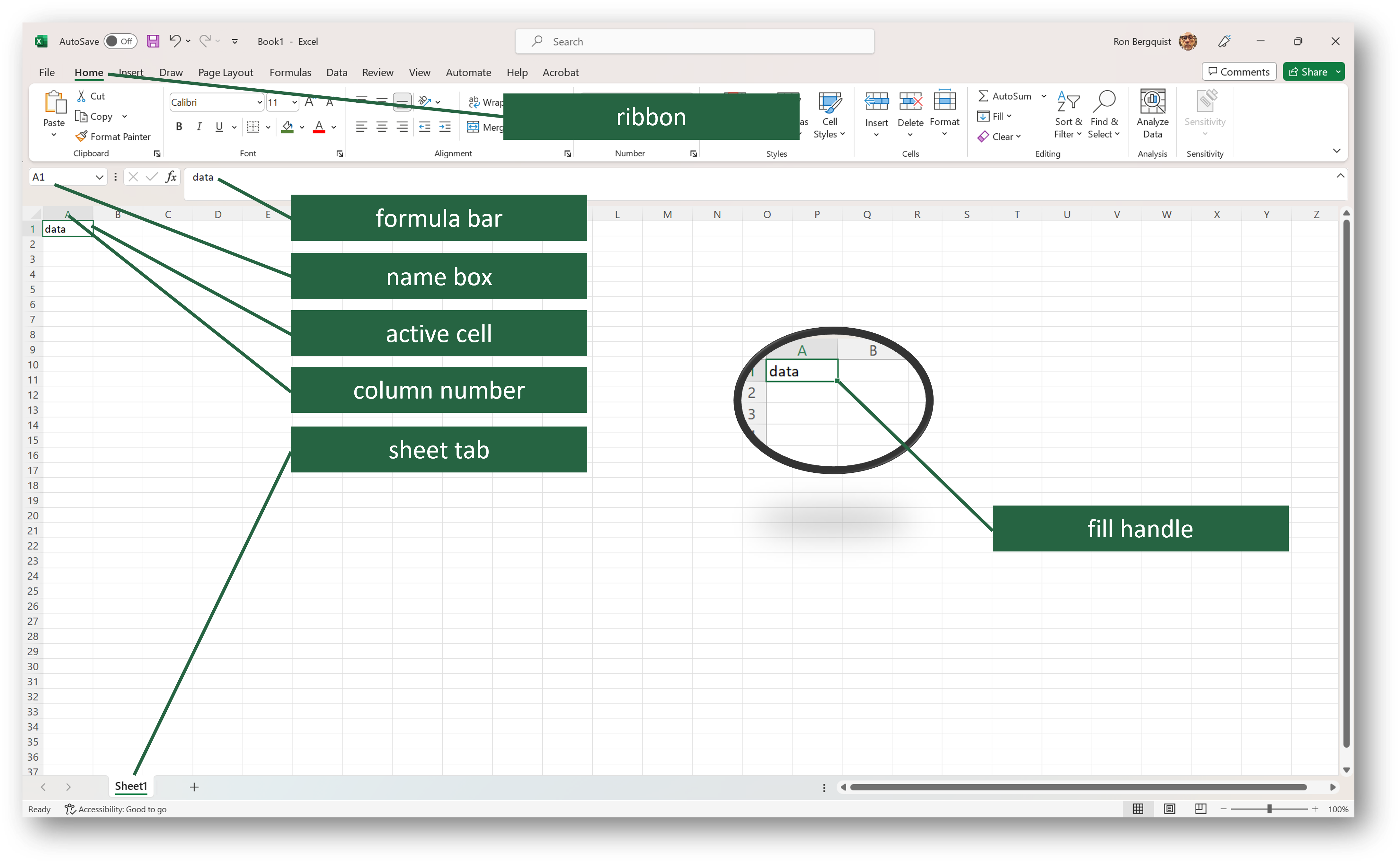
Once you have the value in cell D2, you can use the fill handle and drag down the function from D2 to D84. The function will continue to match the value in the relative column E cell to the absolute values in cells F4 through F11 on the 06-Calendars worksheet and return the related value from cells G4 through G11 and place them in cells D2 through as far as you drag down the function.

Note, when using the fill handle, you drag down all the cell, to include the color formatting of the cell as well as the function within the cell.

We won't do it, but there is also XLOOKUP

To quote an excellent source on the topic ...

XLOOKUP is everything VLOOKUP is and much more.

Here's a fairly robust tutorial on XLOOKUP.