Tools for Information Literacy
Pull data from a second worksheet into a formula on a defferent worksheet
Facility with functions and formatting of the resultant data
- Insert a new worksheet, place it fifth in the sequence of worksheets, and name it 05-Summary.
-
On the 05-Summary worksheet,
in cell B4 enter the words "Highest Foreign Born Percentage in Alabama counties."
In cell K4, insert a function that will return the highest ForeignBornPct from the data about Alabama counties (rows AI4 through AI71) on the 01-Format worksheet. (the cell references are A"eye"4 through A"eye"71) on the 01-Format worksheet. -
On the 05-Summary worksheet,
in cell B5 enter the words "Earliest Foundation Date."
In cell K5 insert a function that will return the foundation date from the data in the FC = Foundation century column (that would be column G) on the 02-Conditional Formatting worksheet. -
On the 05-Summary worksheet,
in cell B6 enter the words "Number of Navy programs in North Carolina".
In cell K6, display the number of programs for which the Navy is the Organization (column F) and North Carolina is the State Country Title (column H).
Find the data on the 13-pivot table data worksheet.
Use your help tool to find the right function.
back to top
facility with formulas ...
... by pulling vectored data from two different worksheets into a new formula
-
Copy cells A5 through A56 from the 16-chart 02 worksheet.
Paste these cells into cells B7 through B58 on the 05-Summary worksheet.
Then, in cell D7, insert a formula that will draw values from two other worksheets.
The formula should divide Alabama's Y1991 values from the 17-medicaid expenditures worksheet (cell G2) by Alabama's Y1991 from the 18-medicaid aggregate worksheet (cell G10).
Remember, this is a formula, not a function.
Then we will demonstrate cell formatting skills based on the type of data the cells contain
-
Once you have created the formula,
format the cell to display percentages to two decimal places.
Remember to format the output of all functions and formulas so that the numbers are displayed as the type of number they are.
-
Once you have formatted the data in the cell,
drag the cell down the column to apply the same formula and formatting for all state rows
back to top
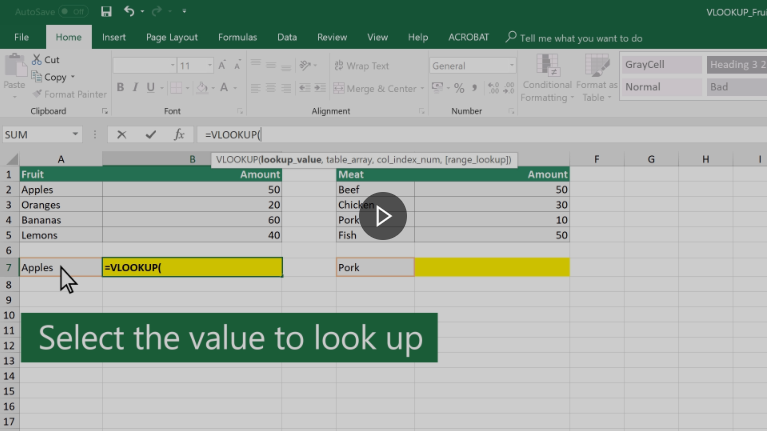
VLOOKUP is an Excel function to lookup and retrieve data from a specific column in table.
It is an Excel way to do what SQL can do with a relational database.
What is VLOOKUP?
It's an Excel function that one may use when one needs to find things in a table or a range by row. For example, look up a price of an automotive part by the part number, or find an employee name based on their employee ID.
In its simplest form, the VLOOKUP function says:
=VLOOKUP(What you want to look up, where you want to look for it, the column number in the range containing the value to return, return an Approximate or Exact match – indicated as 1/TRUE, or 0/FALSE).
back to top
Still using your downloaded workbook ...
We will demonstrate practice with the VLOOKUP function
In this workbook, composed of two worksheets, we want to use a lookup table on the 06-Calendars worksheet to populate data in column D on 12-Spring 2021 Class Schedule worksheet
- select cell D2 on the 07-Fall 2020 Class Schedule
- in the formula bar, insert this formula
(use your CNTL+C or CMD+C to copy it from this web page, and your CNTL+V or CMD+V to paste it in the cell)
=VLOOKUP(E2,'06-Calendars'!$F$4:$G$11,2,FALSE)
This means
- the value in this cell equals
- the value you will find when you use this function to
- compare the value in the same line and one cell to the right on this worksheet,
- to the values in the array of cells on the 06-Calendars worksheet in the absolute range of cells from cell F4 through G11,
- where it will look for a value that matches the value in cell E2 in this worksheet in absolute locations $F$4 through $F$11 on the Calendars worksheet,
- and find the value that resides in the absolute locations $G$4 through $G$11 on the 06-Calendars worksheet,
- D2 on the 07-Fall 2020 Class Schedule worksheet is a vector, a relative location. When you drag down the value in the cell, the vector in the function will continue to look for values in cells in column E and one cell to the right of the function
- The $ before the column and row in the value locks the cells on the 06-Calendars worksheet that the VLookup will use to populate the cells that contain the function
- Without the $, the values would be vectors; with them the values remain in the range of cells you want to use
- and insert that value back into this cell
Once you have the value in cell D2, you can use the fill handle and drag down the function from D2 to D84. The function will continue to match the value in the relative column E cell to the absolute values in cells F4 through F11 on the 06-Calendars worksheet and return the related value from cells G4 through G11 and place them in cells D2 through as far as you drag down the function.
Note, when using the fill handle, you drag down all the cell, to include the color formatting of the cell as well as the function within the cell.